Machine Learning

Decision Tree Algorithms

Sakeef M. Karim
New York University


CONSORTIUM ON ANALYTICS FOR DATA-DRIVEN DECISION-MAKING

Roadmap

What We’ll Cover Today

• What decision trees refer to in the world of supervised learning

• Different types of decision tree models

  • Single decision tree estimators
  • Decision tree ensembles—e.g., random forests and gradient boosting

• Some key terms or concepts we should know before fitting decision tree algorithms—inclusive of leaves, pruning and bagging

• How to grow random forests in Python

What Are Decision Trees?

Decision Trees in the Wild

Image can be retrieved here.

• To put it simply, decision trees are tree-like flowcharts that connect decisions to potential outcomes—i.e., by visualizing the pathways that link our choices to results in the face of uncertainty, chance events etc.

• We can think about decision trees as a series of conditional (if/else) statements:

  • Creating coding rules for ethnographic data.
  • Deciding whether to wear shirt \(x\) or \(y\) before heading outside to face the world.

The Tennis Example

Are we going to play tennis today? Let’s think through the different possibilities.

• Rules
• A Decision Tree

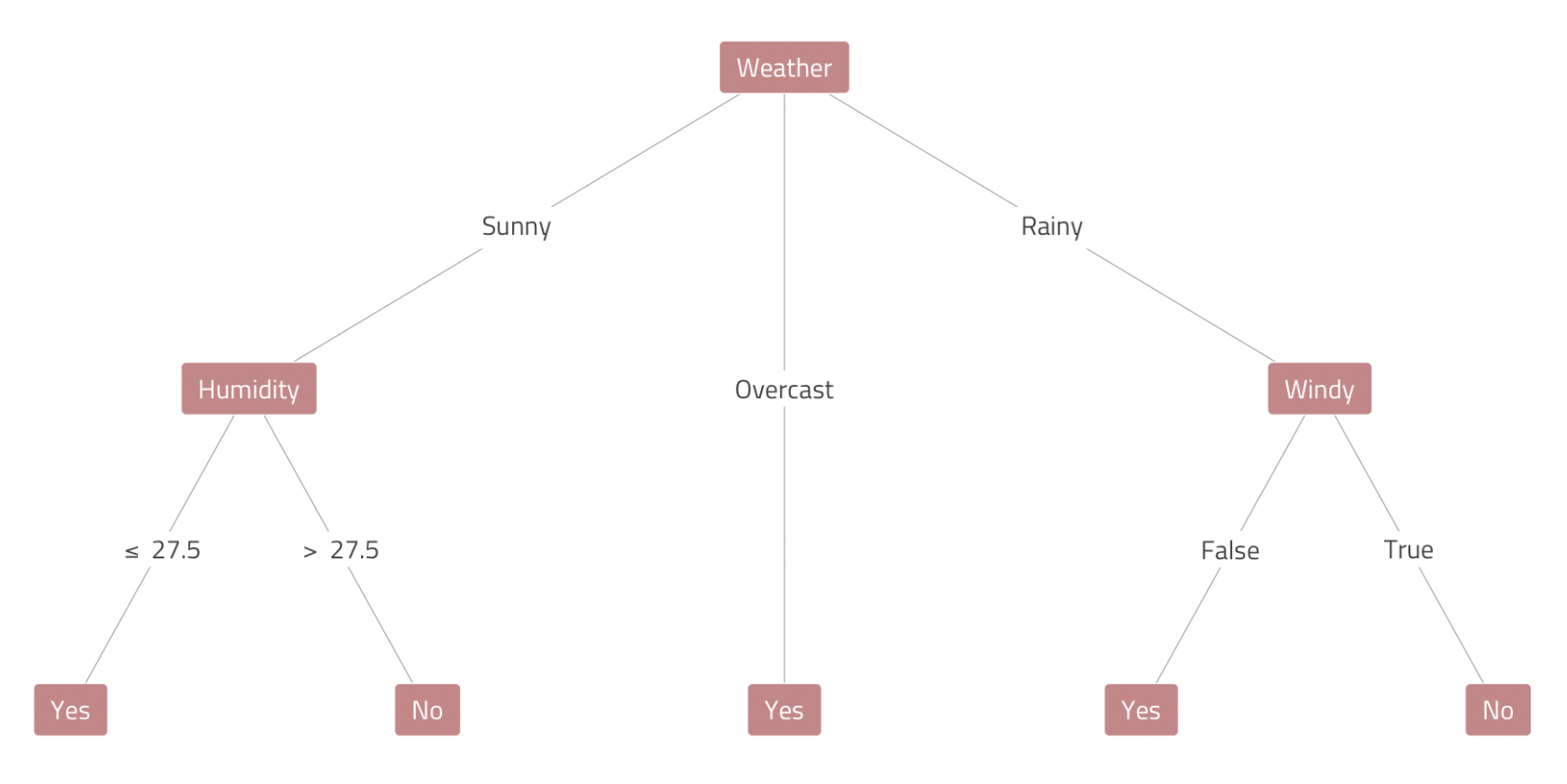
1. If there is a fair bit of cloud cover (i.e., overcast conditions), we’re playing tennis.

2. If it’s sunny, we’ll play tennis—but only if it’s \(\le\) 27.5^o C with humidity.

3. If it’s raining, we’ll play tennis—but only if it’s not windy.

Decision Trees in Machine Learning

• In the world of SML, tree-based algorithms apply the logic of decision trees to resolve regression and classification problems.

• To make predictions, decision tree models take an unseen data point on a journey trough the feature space—or pathways that can lead to different endpoints (terminal nodes) depending on the observation’s features.

• To generate the tree diagram on the left—and explore decision tree estimators for the first time in Python —click here.

The Baseball Example

The following example comes from Introduction to Statistical Learning.

Objective

Use a decision tree to predict a baseball player’s salary using data from ’86.

Data

ISLR2::Hitters %>% rownames_to_column(var = "Player") %>% as_tibble()

# A tibble: 322 × 21
   Player    AtBat  Hits HmRun  Runs   RBI Walks Years CAtBat CHits CHmRun CRuns
   <chr>     <int> <int> <int> <int> <int> <int> <int>  <int> <int>  <int> <int>
 1 -Andy Al…   293    66     1    30    29    14     1    293    66      1    30
 2 -Alan As…   315    81     7    24    38    39    14   3449   835     69   321
 3 -Alvin D…   479   130    18    66    72    76     3   1624   457     63   224
 4 -Andre D…   496   141    20    65    78    37    11   5628  1575    225   828
 5 -Andres …   321    87    10    39    42    30     2    396   101     12    48
 6 -Alfredo…   594   169     4    74    51    35    11   4408  1133     19   501
 7 -Al Newm…   185    37     1    23     8    21     2    214    42      1    30
 8 -Argenis…   298    73     0    24    24     7     3    509   108      0    41
 9 -Andres …   323    81     6    26    32     8     2    341    86      6    32
10 -Andre T…   401    92    17    49    66    65    13   5206  1332    253   784
# ℹ 312 more rows
# ℹ 9 more variables: CRBI <int>, CWalks <int>, League <fct>, Division <fct>,
#   PutOuts <int>, Assists <int>, Errors <int>, Salary <dbl>, NewLeague <fct>

The Baseball Example (cont.)

• Key Variables
• The Decision Tree
• Segmenting the Feature Space

Image can be retrieved here.

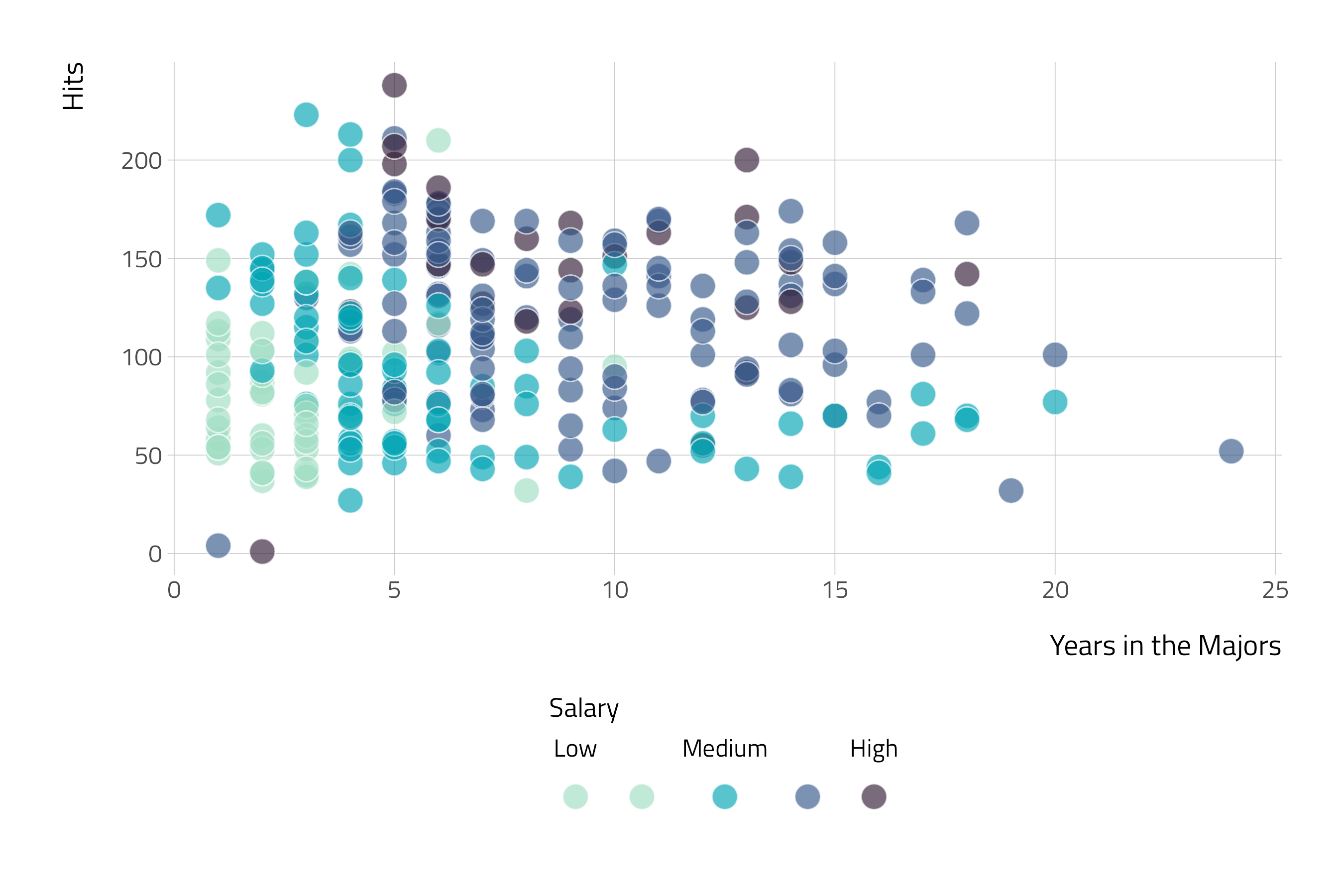
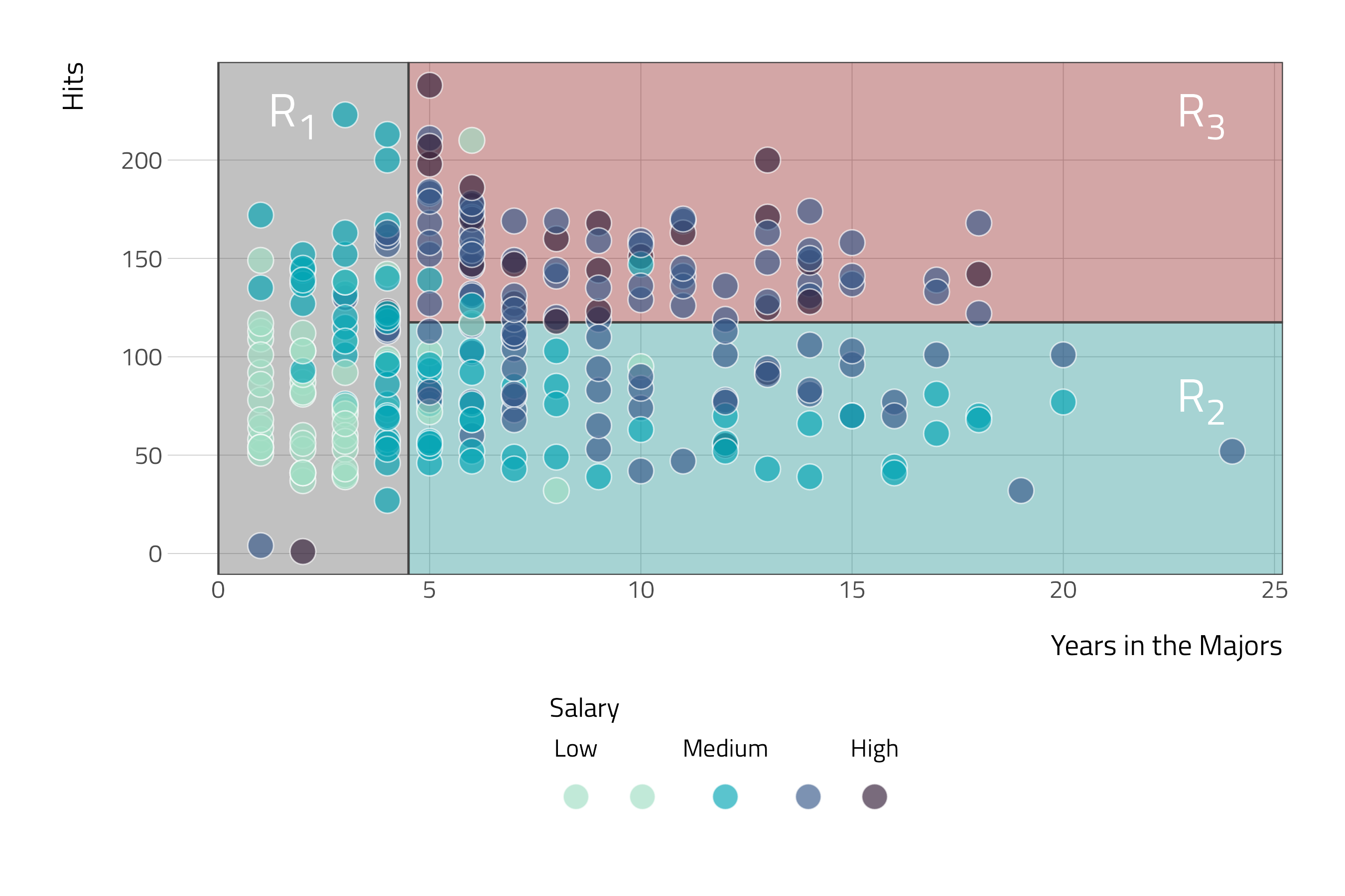
• Here, the feature space is being stratified or segmented into three distinct regions:

  • \(R_1\) = {\(X\) | Years \(<\) 4.5}
  • \(R_2\) = {\(X\) | Years \(\ge\) 4.5, Hits \(<\) 117.5}
  • \(R_3\) = {\(X\) | Years \(\ge\) 4.5, Hits \(\ge\) 117.5}

The Baseball Example (cont.)

• A “New” Data Point
• Model Prediction

Player	Years	Hits	salary
	8	160

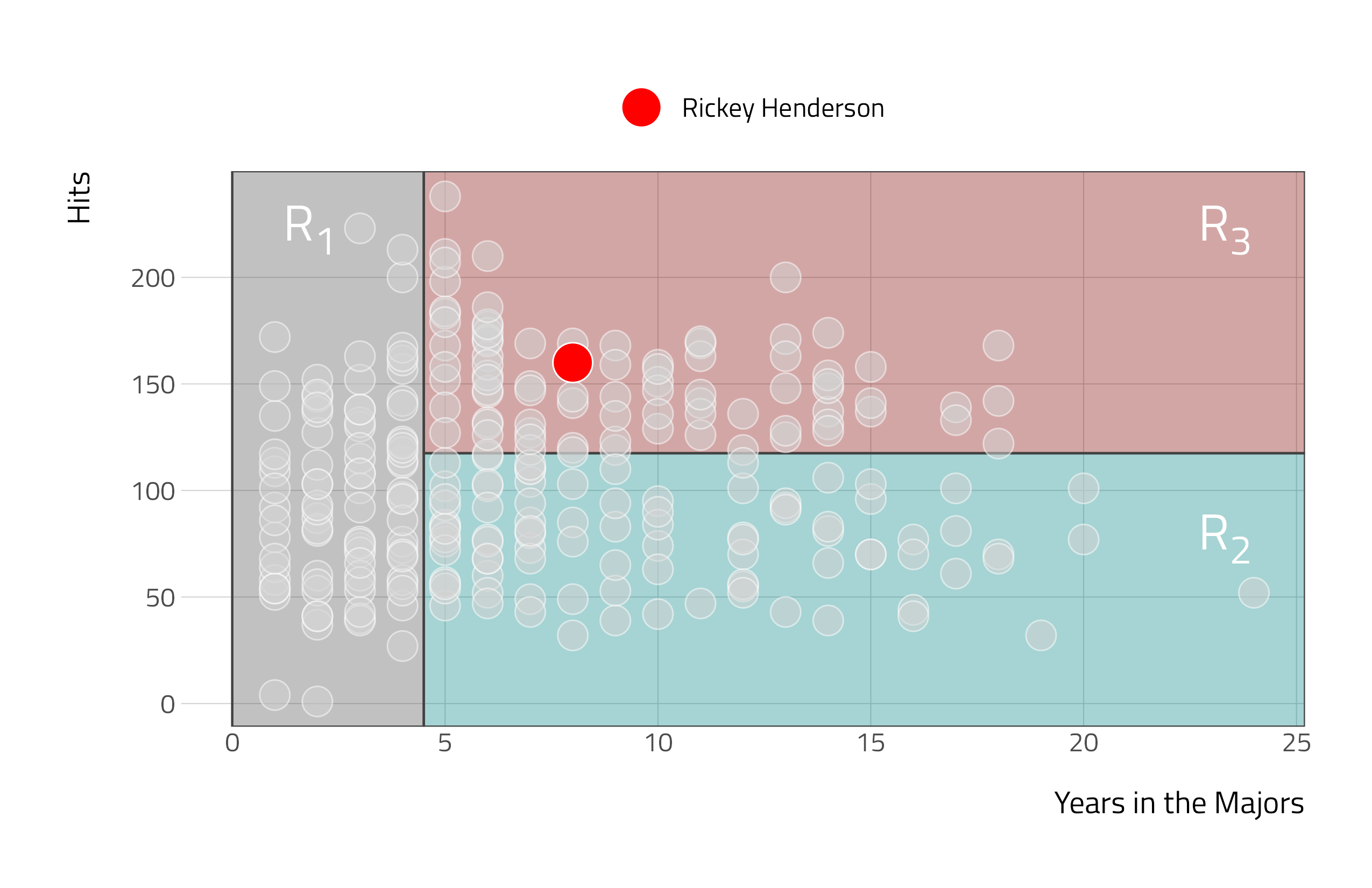
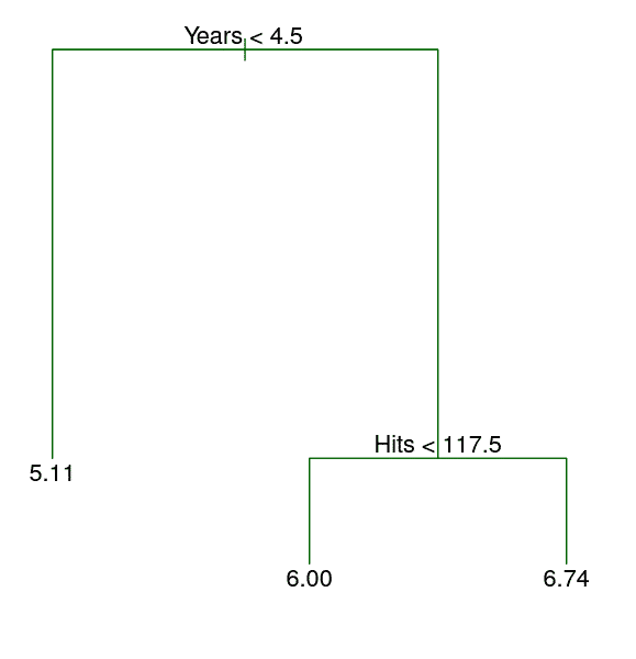
• \(\hat{y}\): 6.74 (logged USD in 1000s)
• Henderson’s salary: 7.42 (logged USD in 1000s)

Single Decision Trees—A Closer Look

Splitting the Feature Space

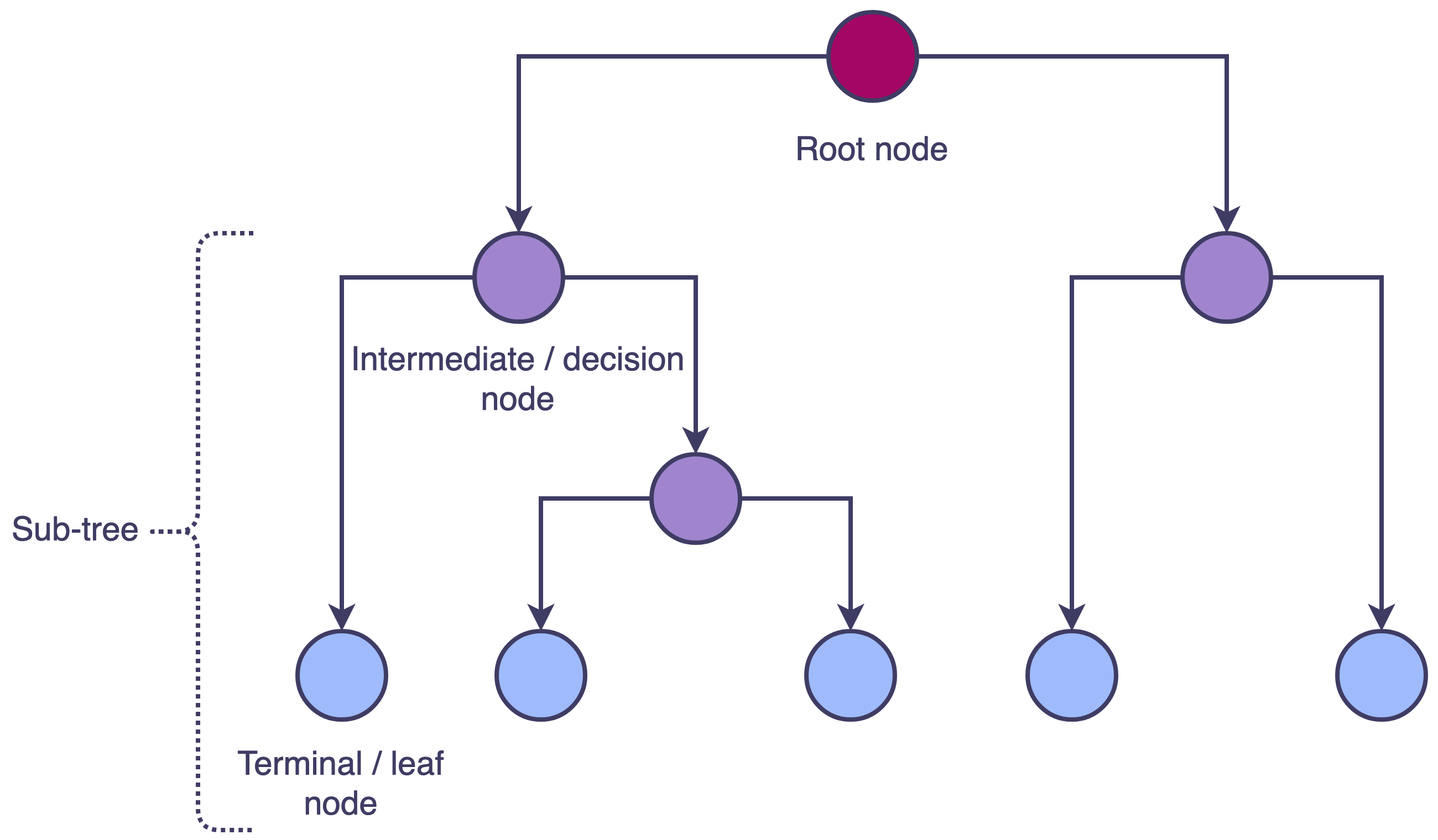
• Decision tree estimators rely on recursive binary splitting to segment the feature space.

  • This procedure begins by selecting the predictor (\(X_j\)) and cutpoint (\(s\), or level of \(X_j\)) such that splitting the feature space into regions {\(X\) | \(X_j\) \(\le\) \(s\)} and {\(X\) | \(X_j\) \(>\) \(s\)} leads to the largest possible reduction in a loss function.

  • The process is then repeated—i.e., by finding the feature and cutpoint that yields the largest possible reduction in a loss function within the two new regions.

  • The algorithm generates more splits or branches until a stopping criterion is reached: e.g., tree depth.

  • Overall, this procedure is top-down and greedy.

Tuning Hyperparameters

Single decision trees are relatively easy to interpret and can account for complex interactions linking \(X\) to \(Y\). However, they are prone to overfitting.

To combat variance across samples, analysts can turn to hyperparameter optimization—i.e., by tuning some of the following hyperparameters:

• Maximum Tree Depth refers to the longest path from the root node to a leaf or terminal node.

• Minimum Samples for a Split refers to the minimum number of training samples that must be present for an internal node to be split further.

• Minimum Samples for a Leaf refers to the minimum number of training samples that must be present in both branches of a potential split.

For a refresher on hyperparamter optimization, click here.

Pruning Trees

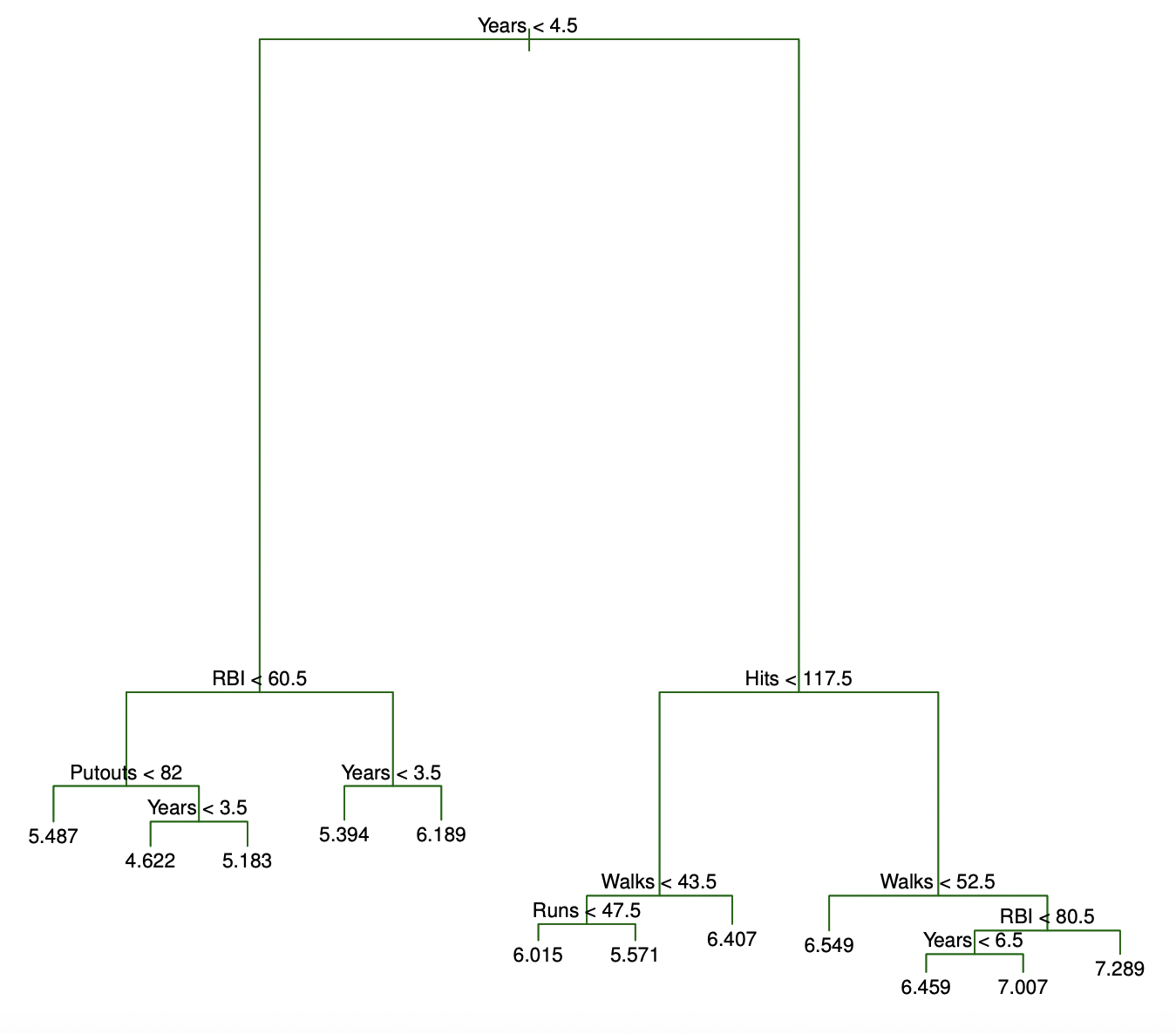
• Beyond tuning a decision tree’s hyperparameters, analysts can combat overfitting by leveraging cost complexity pruning—here are the steps:

  • Grow a very large decision tree, \(T_0\).
  • Supply different values of the penalty parameter \(\alpha\)—each value corresponding to a less complex subtree \(T \subset T_0\).
  • Use cross-validation to find optimal \(\hat{\alpha}\) value.
  • Select the subtree \(T \subset T_0\) corresponding to the optimal \(\hat{\alpha}\) value.

Decision Tree Ensembles

Bagging and Random Forests

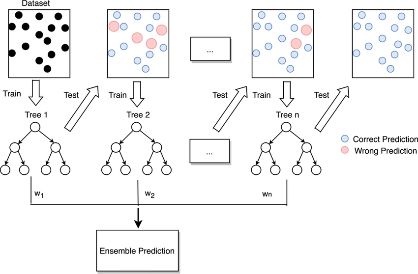
If we combine the results of many decision trees—or grow an ensemble of tree-based models—the predictive power of our decision tree estimators can be significantly enhanced.

• Bootstrap Aggregation
• Random Forests

Image can be retrieved here.

• Bootstrap aggregation—or bagging—is an ensemble learning procedure that is implemented as follows:
  • We repeatedly sample from training data with replacement—i.e., bootstrapping—until we have \(B\) synthetic (and independent) datasets with the same dimensions as our training data.
  • We grow \(B\) large decision trees on each of the \(B\) (e.g., 1000) datasets.
    
  • We aggregate predictions from each of the \(B\) decision trees (via averaging or voting) to generate our final prediction, \(\hat{f}_{bag}(x)\).
    
• See Canvas for details on out-of-bag scores for ensemble trees.

• Random forest algorithms blend bagging and feature randomness to ensure that decision trees within the ensemble are uncorrelated.

• Within each of the \(B\) decision trees, the random forest algorithm only considers a random subset, \(m\), of the \(p\) features (e.g., \(m \approx \sqrt{p}\)) at each decision point.

• Like before, we aggregate predictions from each of the \(B\) decision trees (via averaging or voting) to generate our final prediction, \(\hat{f}_{bag}(x)\).

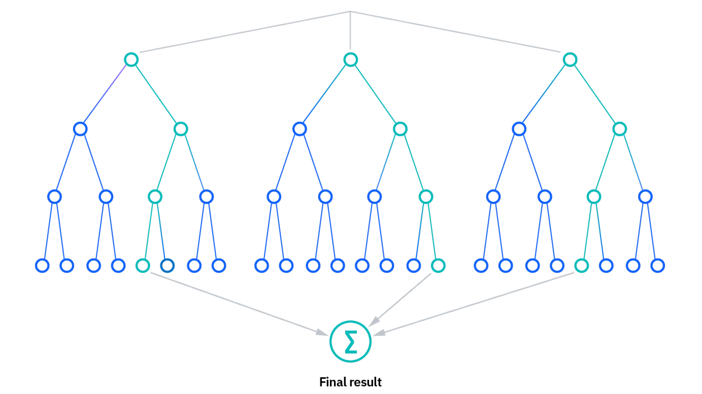
Image can be retrieved here.

Gradient Boosted Trees

• Boosting is another approach to ensemble learning—i.e., where small decision trees (weak learners) are sequentially grown to attack the residuals left over by their predecessors.

• At each boosting stage (or iteration), we slowly improve \(\hat{f}\) by learning to account for some of the residual errors inherited from previous trees.

• For gradient boosted trees, important hyperparameters include \(B\) (the number of trees in the ensemble) and \(\lambda\)—the shrinkage parameter.

• Ultimately, predictions are made by passing observations through the entire ensemble of trees (with each tree weighted by \(\lambda\)).

Image can be retrieved here.

Growing Random Forests

Random Forests in Python

The code snippets embedded below—and their companion Colab Notebook—can be found by clicking here.

Importing Libraries, Loading Data

# Importing pandas to load/wrangle the data, modules from scikit-learn to fit random forest classifier:

import pandas as pd 

from sklearn import metrics

from sklearn.model_selection import train_test_split

from sklearn.ensemble import RandomForestClassifier

# Load input data frame:

penguins = pd.read_stata('https://github.com/sakeefkarim/python_plotting/blob/main/files/palmerpenguins.dta?raw=true')

penguins = penguins.dropna()

Performing Train-Test Split

# Target: 

y = penguins['species']

# Generating input table:

X = penguins.drop(columns = ['species'])

# Adjusting categorical inputs:

adjusted_island = pd.get_dummies(X["island"], drop_first=True)

adjusted_sex = pd.get_dummies(X["sex"], drop_first=True)

# Final set of features:

X = pd.concat([X, adjusted_island, adjusted_sex], axis=1).drop(columns = ['island', 'sex'])

# Train-test split

X_train, X_test, y_train, y_test = train_test_split(X, y, stratify = y, test_size = 0.2, random_state = 416)

Fitting Random Forest Classifier

# Developing random forest classifier with 1000 decision trees:

rf = RandomForestClassifier(n_estimators=1000, max_depth = 5, random_state = 416)

# Fitting model:

rf.fit(X_train, y_train)

# Evaluating out-of-sample performance:  

rf_pred = rf.predict(X_test)

print(metrics.classification_report(rf_pred, y_test))

Keep clicking to move through the code highlights and advance to the next slide.

A Quick Exercise

Using data from {palmerpenguins}, develop a random forest regressor to predict a numeric outcome of interest. Along the way, try to:

1. Settle on the optimal number of estimators (n_estimators) for your classifier using a grid search of possible hyperparameter values for \(B\).
2. Report your algorithm’s out-of-bag score or out-of-sample performance.

The End